45 pivot table excel multiple row labels
support.microsoft.com › en-us › officeTutorial: Extend Data Model relationships using Excel, Power ... Notice that the Power Pivot window shows all the tables in the model, including Hosts.Click through a couple of tables. In Power Pivot you can view all of the data that your model contains, even if they aren’t displayed in any worksheets in Excel, such as the Disciplines, Events, and Medals data below, as well as S_Teams,W_Teams, and Sports. How to make row labels on same line in pivot table? - ExtendOffice In Excel, when you create a pivot table, the row labels are displayed as a compact layout, all the headings are listed in one column. Sometimes, you need to convert the compact layout to outline form to make the table more clearly. This article will tell you how to repeat row labels for group in Excel PivotTable.
This was created by specifying np.mean in the aggregate function and ... Reading multiple headers from a CSV or Excel files can be done by using parameter ... a simple way to group numeric data into bins is via the Pivot Table. Pull the numeric variable into the "row labels". Now right-click on any of the values in this right column and choose "Group". ... In this quiz, we will test you on the basis of the basics of ...
Pivot table excel multiple row labels
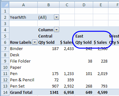
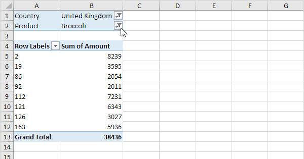
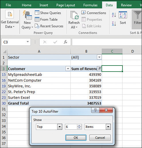
Excel: How to Apply Multiple Filters to Pivot Table at Once Example: Apply Multiple Filters to Excel Pivot Table. Suppose we have the following pivot table in Excel that shows the total sales of various products: Now suppose we click the dropdown arrow next to Row Labels, then click Label Filters, then click Contains: And suppose we choose to filter for rows that contain "shirt" in the row label: › excel-pivot-table-filtersExcel Pivot Table Date Filters - Contextures Excel Tips Jun 22, 2022 · Pivot Table in Compact Layout. If your pivot table is in Compact Layout, all of the Row fields are in a single column. The column heading says "Row Labels". To choose the pivot field that you want to filter, follow these steps: In the pivot table, click the drop down arrow on the Row Labels heading; In the Select Field box, slick the drop down ... Automatic Row And Column Pivot Table Labels - How To Excel At Excel Select the data set you want to use for your table The first thing to do is put your cursor somewhere in your data list Select the Insert Tab Hit Pivot Table icon Next select Pivot Table option Select a table or range option Select to put your Table on a New Worksheet or on the current one, for this tutorial select the first option Click Ok
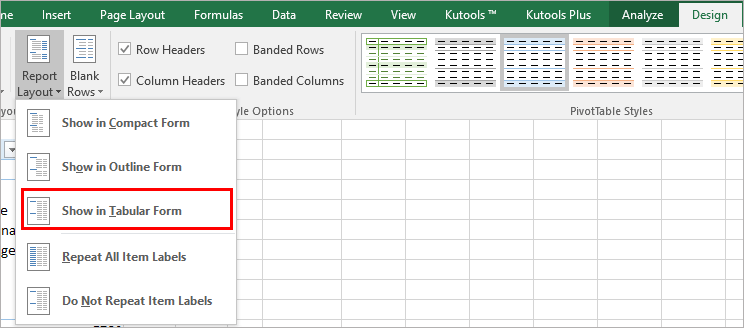
Pivot table excel multiple row labels. Pivot Table Row Labels In the Same Line - Beat Excel! Then navigate to "Layout & Print" tab and click on "Show item in tabular form" option. Do this procedure also for "Dealer" field and your table will look like this: If you also want dealer names to repeat on each row, reopen "Dealer field settings and check "Repear item labels" option in "Layout & Print" tab. How to make row labels on same line in pivot table? - ExtendOffice In Excel, when you create a pivot table, the row labels are displayed as a compact layout, all the headings are listed in one column. Sometimes, you need to convert the compact layout to outline form to make the table more clearly. This article will tell you how to repeat row labels for group in Excel PivotTable. Pivot table row labels side by side - Excel Tutorial - OfficeTuts Excel You can copy the following table and paste it into your worksheet as Match Destination Formatting. Now, let's create a pivot table ( Insert >> Tables >> Pivot Table) and check all the values in Pivot Table Fields. Fields should look like this. Right-click inside a pivot table and choose PivotTable Options…. Check data as shown on the image below. How to make row labels on same line in pivot table in excel #ExcelMaster, #PivotTable, #ExcelHow to make row labels on same line in pivot table in excelHow to show multiple rows in pivot table in excel
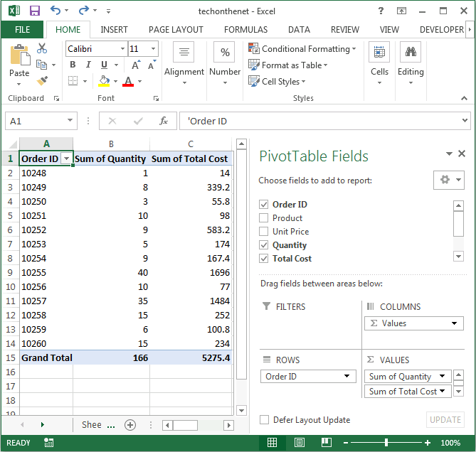
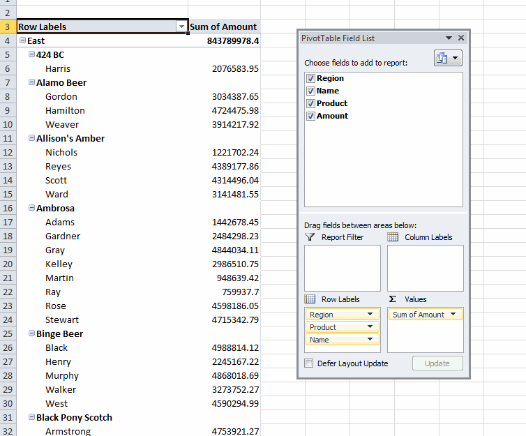
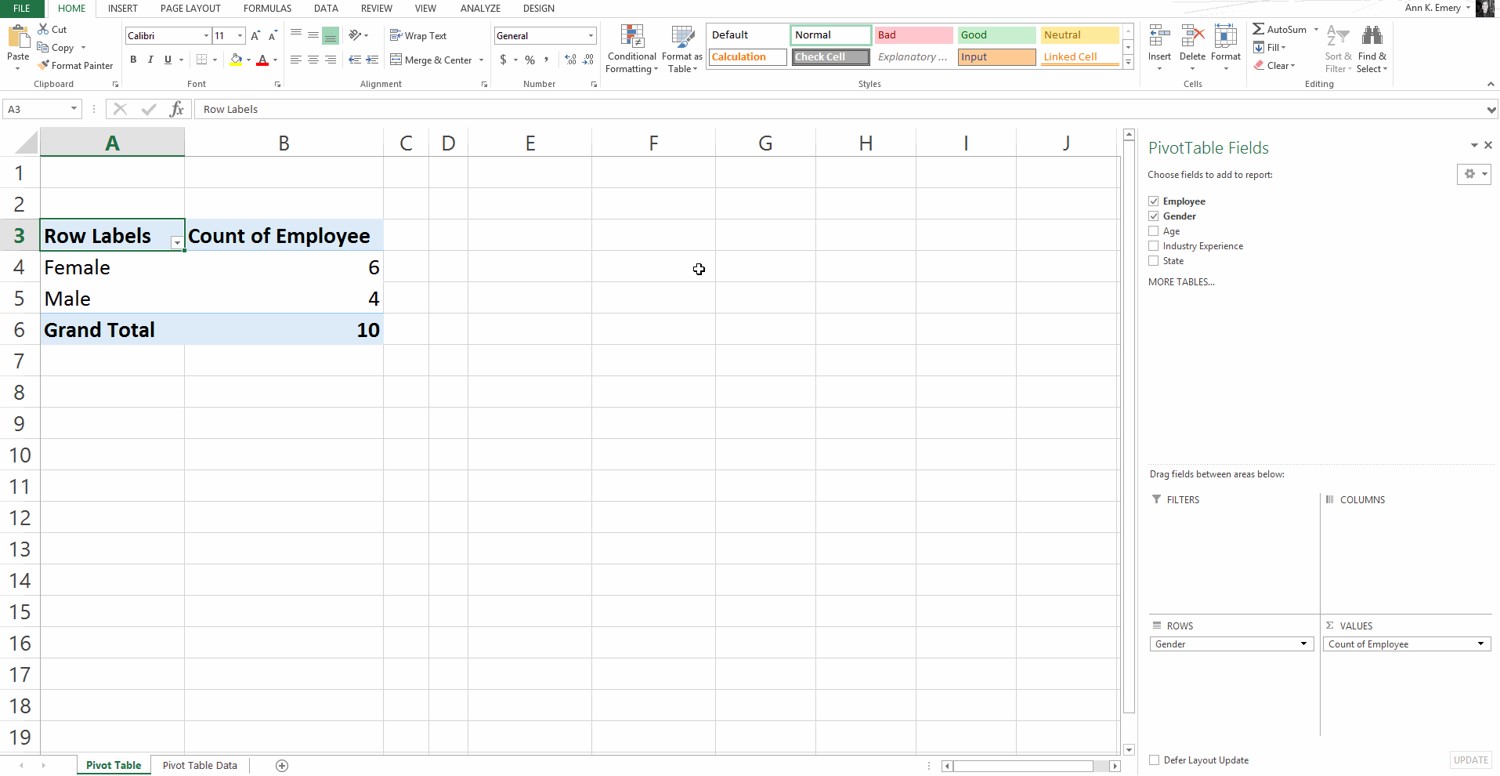
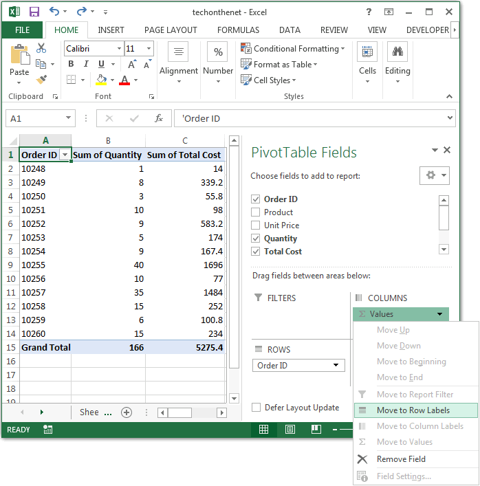
en.wikipedia.org › wiki › Pivot_tablePivot table - Wikipedia Pivot tables are not created automatically. For example, in Microsoft Excel one must first select the entire data in the original table and then go to the Insert tab and select "Pivot Table" (or "Pivot Chart"). The user then has the option of either inserting the pivot table into an existing sheet or creating a new sheet to house the pivot table. Excel Pivot Table with nested rows | Basic Excel Tutorial Insert your pivot table. Click Insert Menu, under Tables group choose PivotTable. 2. Once you create your pivot table, add all the fields you need to analyze data. How to add the fields. Select the checkbox on each field name you desire in the field section. The selected fields are added to the Row Labels area in the layout section. › pivot-table-tips-and-tricks101 Advanced Pivot Table Tips And Tricks You Need To Know Apr 25, 2022 · As a new pivot table user I LOVE this website – very well written! I do have a unique issue I’m hoping to get assistance with. I have a pivot table built out with multiple rows and columns pertaining to new hire information. My boss likes the option to “drill down” and view the source data. How to rename group or row labels in Excel PivotTable? - ExtendOffice Click at the PivotTable, then click Analyze tab and go to the Active Field textbox. 2. Now in the Active Field textbox, the active field name is displayed, you can change it in the textbox. You can change other Row Labels name by clicking the relative fields in the PivotTable, then rename it in the Active Field textbox.
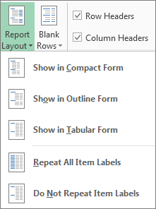
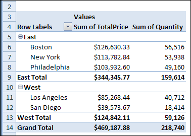
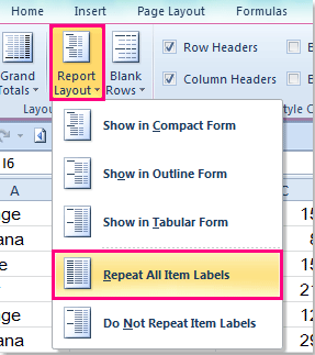
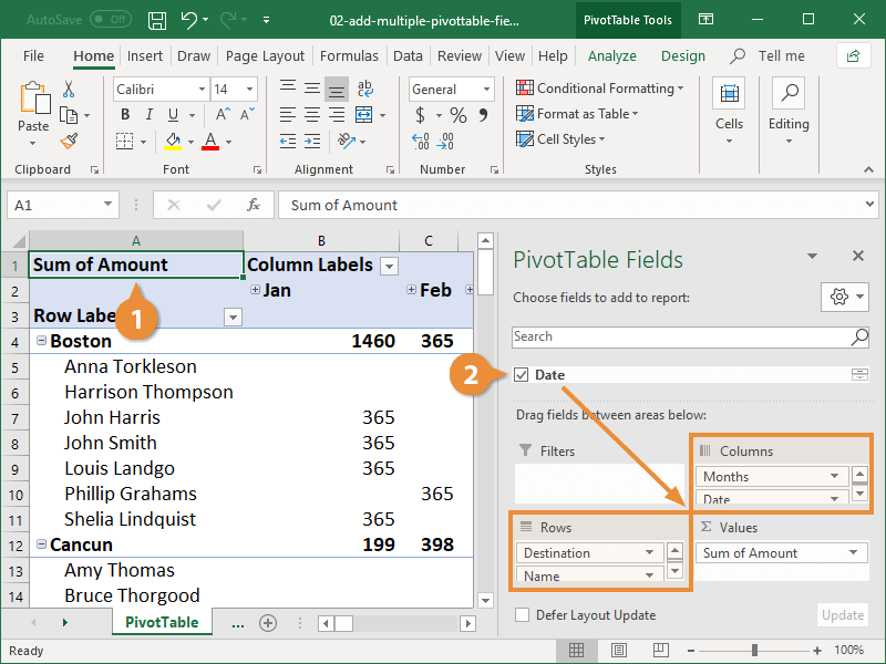
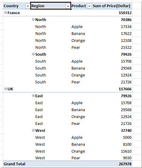
Repeat item labels in a PivotTable - support.microsoft.com Repeating item and field labels in a PivotTable visually groups rows or columns together to make the data easier to scan. For example, use repeating labels when subtotals are turned off or there are multiple fields for items. In the example shown below, the regions are repeated for each row and the product is repeated for each column. How to repeat row labels for group in pivot table? - ExtendOffice Except repeating the row labels for the entire pivot table, you can also apply the feature to a specific field in the pivot table only. 1. Firstly, you need to expand the row labels as outline form as above steps shows, and click one row label which you want to repeat in your pivot table. 2. Multiple row labels on one row in Pivot table - MrExcel Message Board I figured it out - Right click on your pivot table and choose pivot table options/display. Click on "Classic PivotTable layout" Then click on where it is subtotaling your row label and uncheck the subtotal option. D dudeshane0 New Member Joined Oct 23, 2014 Messages 1 Jan 19, 2015 #6 Gerald Higgins said: Multi-row and Multi-column Pivot Table - Excel Start Click OK Once the pivot table sheet is created, just like in the previous example, drag the Category and the Product to the Rows section and the Sales Value to the Values section to get the same Multi-Row pivot table we did in the previous example. Next we want to add a column. We will add the Date to the Column section by dragging the field.
Centre Column Headings in Excel Pivot Table | Excel Pivot Tables
Pivot Table Multiple Row Labels? [SOLVED] - Excel Help Forum then, create a second pivot table that sums the values at the Engineer level. If you need to present this data in a contiguous table, you can create a new Excel table and reference to the pivot table values with formulas (=PivotTableSheet!A1) cheers Register To Reply 09-29-2010, 05:56 AM #6 kopite2002 Registered User Join Date 09-23-2010 Location

How to repeat row labels for group in pivot table?
Just follow the steps given below. Step 1: Be on any of the cells in a Location of Pivot Table: on a new sheet, titled Pivot. Build the table with Item as rows, Helper Column as Values. 5. Insert Slicer for Item (on the PivotTable Analyze tab). Create Helper Cells with GETPIVOTDATA. So here. Step 3. Highlight your cells to create your pivot table. Once you've entered data into your Excel worksheet, and sorted it ...

Excel Pivot Table with multiple columns of data and each data ...
How to Add Rows to a Pivot Table: 9 Steps (with Pictures) - wikiHow Click anywhere in your pivot table. This opens the pivot table editor on the right side of Google Sheets. 3. Click Add under "Rows." It's in the left side of the pivot table editor. A list of fields will expand on the menu. 4. Click the name of the field you want to add as a row.

Pivot Tables Row Labels in Excel 2007 - YouTube
› xlpivot08Excel Pivot Table Multiple Consolidation Ranges Jul 25, 2022 · Pivot Tables > Create > Multiple Sources Pivot Table Multiple Consolidation Ranges. Create a Pivot Table using data from different sheets in a workbook, or from different workbooks, if those tables have identical column structures. Also, see alternatives to multiple consolidation ranges, by using Power Query or a Union Query.

Pivot table row labels in separate columns • AuditExcel.co.za
multiple fields as row labels on the same level in pivot table Excel ... multiple fields as row labels on the same level in pivot table Excel 2016 I am using Excel 2016. I have data that lists product models along with relevant data and also production volumes by month. Part of the relevant data are about 5 common part columns with the part # that applies to each model under the appropriate column.
How to Filter Data in a Pivot Table in Excel
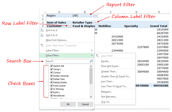
› excelpivottablelabelfiltersHow to Use Excel Pivot Table Label Filters Jun 22, 2022 · The item is immediately hidden in the pivot table. Quickly Hide All But a Few Items. You can use a similar technique to hide most of the items in the Row Labels or Column Labels. Select the pivot table items that you want to keep visible; Right-click on one of the selected items; In the pop-up menu, click Filter, then click Keep Only Selected ...
Repeat item labels in a PivotTable
Duplicate Items Appear in Pivot Table - Excel Pivot Tables In Row 2 of the new column, enter the formula =TRIM(C2). Copy the formula down to the last row of data in the source table. If the source data is stored in an Excel Table, the formula should copy down automatically. Refresh the pivot table ; Remove the City field from the pivot table, and add the CityName field to replace it. _____
How to repeat row labels for group in pivot table?
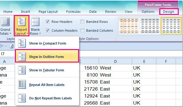
Pivot table row labels in separate columns • AuditExcel.co.za The issue here is simply that the more recent versions of Excel use this as the default report format. Our preference is rather that the pivot tables are shown in tabular form (all columns separated and next to each other). You can do this by changing the report format. So when you click in the Pivot Table and click on the DESIGN tab one of the ...
How to make row labels on same line in pivot table?
› pivot-tables › structure-pivotHow to Setup Source Data for Pivot Tables - Unpivot in Excel Jul 19, 2013 · The correct vs. incorrect structure for pivot table source data. Why it is important to understand this. How to convert your reports into the right structure using formulas (free sample workbook). Data Table Structure. The first step to creating a pivot table is setting up your data in the correct table structure or format.
How to make row labels on same line in pivot table?
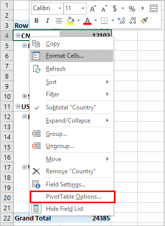
How to make row labels on same line in pivot table? - ExtendOffice Make row labels on same line with PivotTable Options You can also go to the PivotTable Options dialog box to set an option to finish this operation. 1. Click any one cell in the pivot table, and right click to choose PivotTable Options, see screenshot: 2.
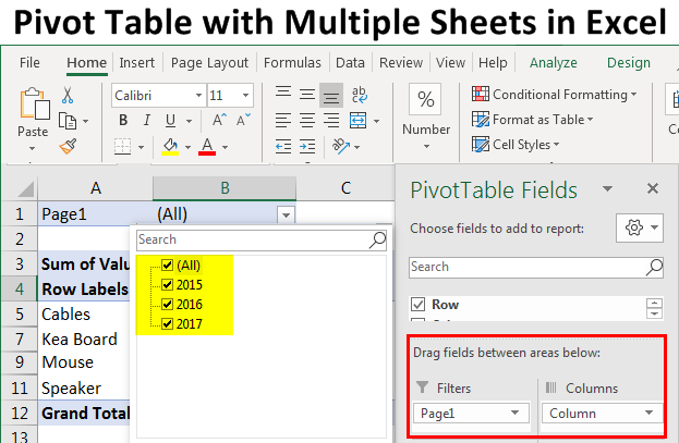
Pivot Table with Multiple Sheets in Excel | Combining ...
Remove PivotTable Duplicate Row Labels [SOLVED] Re: Remove PivotTable Duplicate Row Labels. Sometimes when the cells are stored in different formats within the same column in the raw data, they get duplicated. Also, if there is space/s at the beginning or at the end of these fields, when you filter them out they look the same, however, when you plot a Pivot Table, they appear as separate ...
Instructions for Sorting a Pivot Table by Two Columns | Excelchat
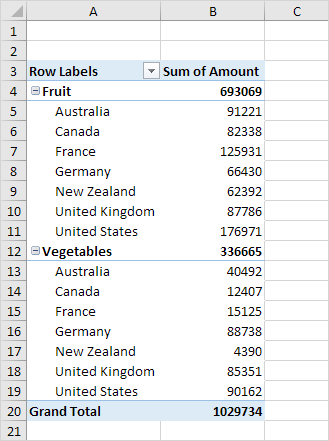
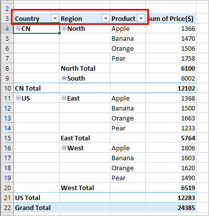
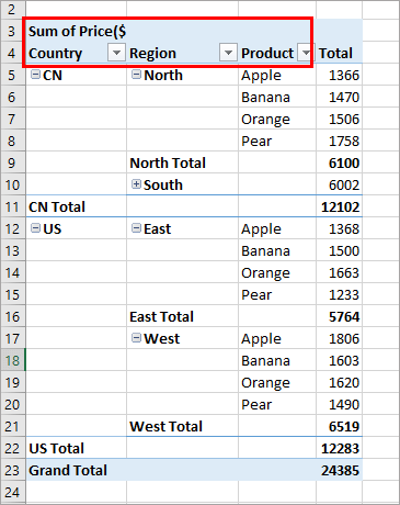
Multi-level Pivot Table in Excel (Easy Tutorial) Below you can find the multi-level pivot table. Multiple Value Fields First, insert a pivot table. Next, drag the following fields to the different areas. 1. Country field to the Rows area. 2. Amount field to the Values area (2x). Note: if you drag the Amount field to the Values area for the second time, Excel also populates the Columns area.
MS Excel 2013: Display the fields in the Values Section in a ...
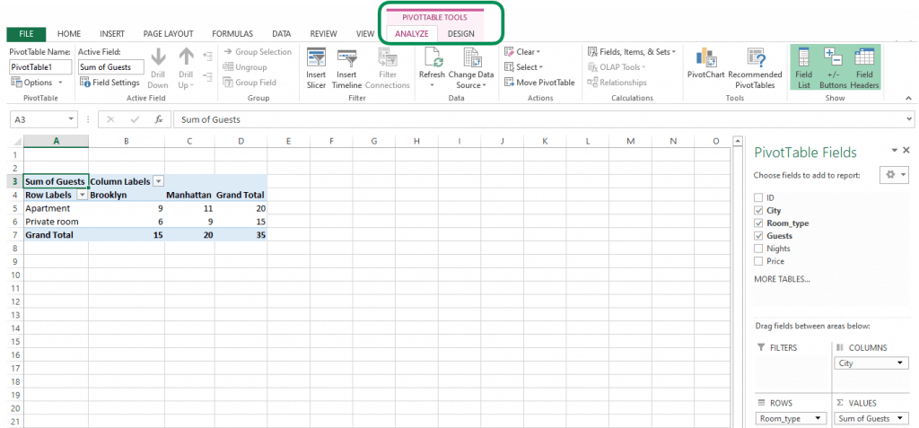
How to add multiple fields into a pivot table in Excel? Step 4. In order to populate the pivot table, click on the checkbox beside the field names. Refer to below screenshot for the same. Step 5. Now, click on the checkboxes beside the field names to make a multi filed level pivot table. The select descriptive fields are automatically added under the Rows category.

Automatic Row And Column Pivot Table Labels
Automatic Row And Column Pivot Table Labels - How To Excel At Excel Select the data set you want to use for your table The first thing to do is put your cursor somewhere in your data list Select the Insert Tab Hit Pivot Table icon Next select Pivot Table option Select a table or range option Select to put your Table on a New Worksheet or on the current one, for this tutorial select the first option Click Ok
Create Multiple Subtotals in a Pivot Table | Excel Pivot Tables
› excel-pivot-table-filtersExcel Pivot Table Date Filters - Contextures Excel Tips Jun 22, 2022 · Pivot Table in Compact Layout. If your pivot table is in Compact Layout, all of the Row fields are in a single column. The column heading says "Row Labels". To choose the pivot field that you want to filter, follow these steps: In the pivot table, click the drop down arrow on the Row Labels heading; In the Select Field box, slick the drop down ...
How to repeat row labels for group in pivot table?
Excel: How to Apply Multiple Filters to Pivot Table at Once Example: Apply Multiple Filters to Excel Pivot Table. Suppose we have the following pivot table in Excel that shows the total sales of various products: Now suppose we click the dropdown arrow next to Row Labels, then click Label Filters, then click Contains: And suppose we choose to filter for rows that contain "shirt" in the row label:
The Pivot table tools ribbon in Excel
Multi-level Pivot Table in Excel (Easy Tutorial)
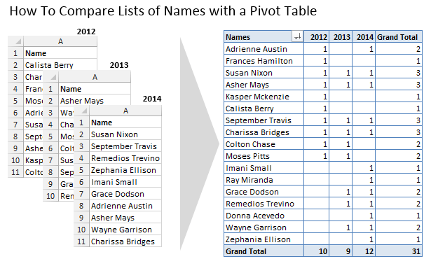
How To Compare Multiple Lists of Names with a Pivot Table ...

Pivot Table Row Labels In the Same Line - Beat Excel!

Excel pivot table shows only when rows have multiple other ...
Multiple Row Filters in Pivot Tables
Pivot Table Tips | Exceljet
Grouping, sorting, and filtering pivot data | Microsoft Press ...
Group or ungroup data in a PivotTable

Permanently Tabulate Pivot Table Report & Repeat All Item ...

How to Delete a Pivot Table in Excel (Easy Step-by-Step Guide)

Pivot table row labels in separate columns • AuditExcel.co.za

How to Create Pivot Table in Excel - All Things How

Making Report Layout Changes | Customizing an Excel 2013 ...

Fix Excel Pivot Table Missing Data Field Settings
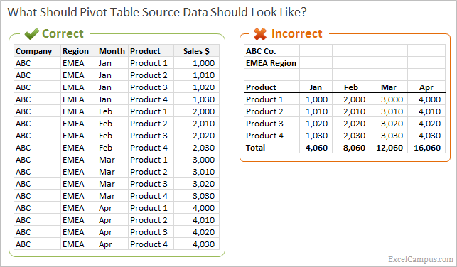
How to Setup Source Data for Pivot Tables - Unpivot in Excel
How To Manage Big Data With Pivot Tables

Remove Group Heading Excel Pivot Table - Stack Overflow
Multi-level Pivot Table in Excel (Easy Tutorial)
Repeating Values in Pivot Tables – Daily Dose of Excel
Instructions for Sorting a Pivot Table by Two Columns | Excelchat

Excel: How to Apply Multiple Filters to Pivot Table at Once ...
Add Multiple Columns to a Pivot Table | CustomGuide
How to Save Time and Energy by Analyzing Your Data with Pivot ...
How to make row labels on same line in pivot table?
MS Excel 2013: Display the fields in the Values Section in a ...
How to make row labels on same line in pivot table?

Excel pivot table shows only when rows have multiple other ...
How to repeat row labels for group in pivot table?
Post a Comment for "45 pivot table excel multiple row labels"